Total Variation Distance
The GRI is built on Total Variation Distance (TVD), one of the most fundamental metrics in probability theory. For discrete distributions \(P\) and \(Q\) over a shared set of categories:
\[
\text{TVD}(P, Q) = \frac{1}{2} \sum_{i=1}^{k} |p_i - q_i|
\]
TVD has several properties that make it ideal for representativeness measurement:
- Bounded: Always in \([0, 1]\), enabling direct comparison across dimensions and surveys
- Metric: Satisfies non-negativity, symmetry, and the triangle inequality
- Interpretable: Equals the maximum difference in probability assigned to any event
- Distribution-free: No parametric assumptions required
- Additive sensitivity: Every stratum contributes proportionally to the total distance
GRI Calculation
The GRI is defined as the complement of TVD:
\[
\text{GRI}(p, q) = 1 - \text{TVD}(p, q) = 1 - \frac{1}{2} \sum_{i=1}^{k} |p_i - q_i|
\]
This maps to a 0–1 scale where 1.0 = perfect match and 0.0 = complete mismatch.
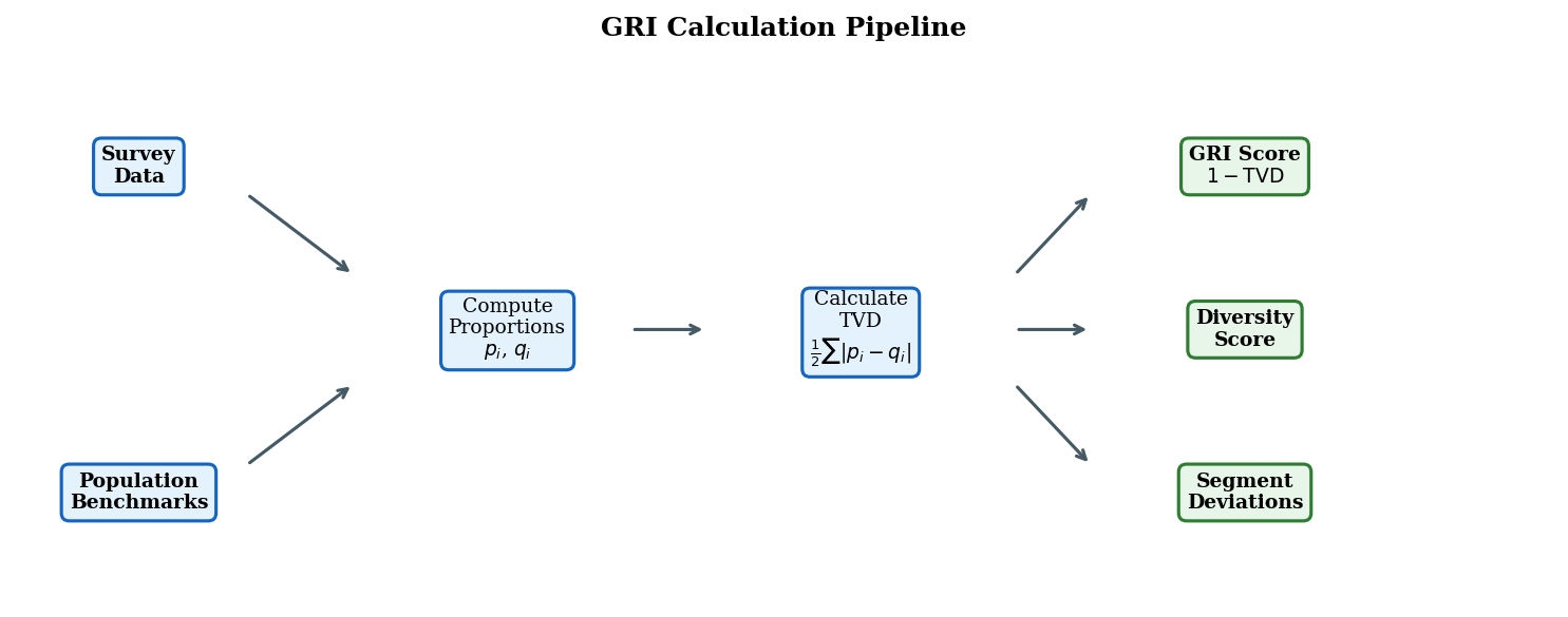
Calculation Pipeline
Inputs:
- Survey data — one row per respondent with demographic columns (country, gender, age group, religion, environment type)
- Population benchmarks — global demographic proportions from authoritative sources
Process:
- Cross demographic columns to form strata (e.g., “India x Female x 25–34”)
- Compute sample proportions \(p_i\) for each stratum
- Look up population proportions \(q_i\) from benchmarks
- Calculate TVD and convert to GRI
Diversity Score
The GRI captures how closely the sample matches the population, but not how many population segments are represented at all. The Diversity Score fills this gap:
\[
\text{Diversity} = \frac{|\{i : p_i > 0 \text{ and } q_i \geq X\}|}{|\{i : q_i \geq X\}|}
\]
where \(X = \frac{1}{2N}\) is a dynamic relevance threshold that scales with sample size. This measures the fraction of meaningfully-sized population strata that appear at least once in the sample.
Multi-Dimensional Scorecard
The GRI is computed across 13 dimensions organized in three tiers:
Primary Dimensions (intersectional)
These combine geography with demographics, producing the finest-grained assessment:
| Country x Gender x Age |
2,699 |
UN WPP 2023 |
| Country x Religion |
1,607 |
Pew GLS 2010 |
| Country x Environment |
449 |
UN WUP 2018 |
Single-Axis Dimensions (marginal)
Assess one demographic factor at a time:
- Country, Continent, Religion, Environment, Age Group, Gender
Each dimension tells a different story. A survey might achieve strong continental representation (GRI = 0.88) while poorly representing the Country x Gender x Age intersection (GRI = 0.37)—the scorecard makes these trade-offs transparent.
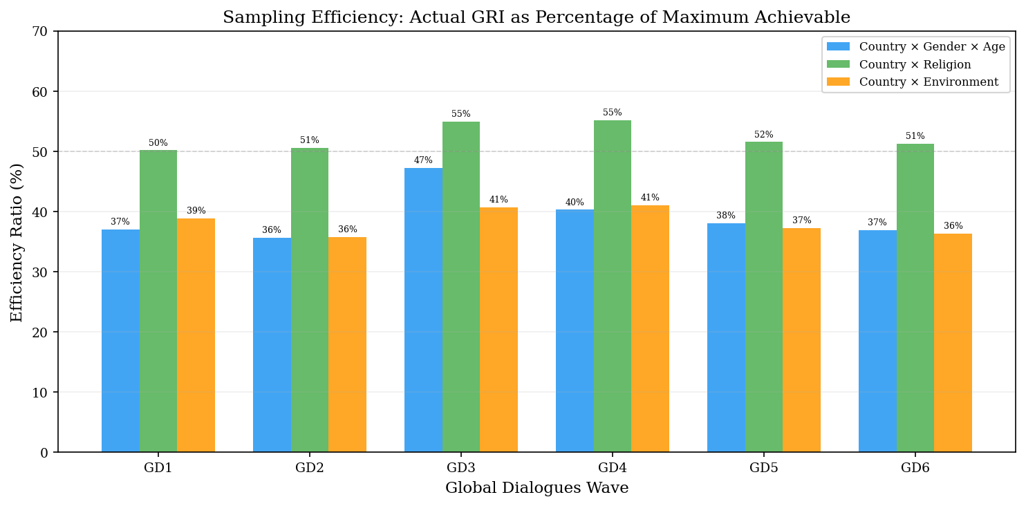
Maximum Achievable Scores
With thousands of strata and finite samples, perfect GRI scores are mathematically impossible. We use Monte Carlo simulation to estimate the maximum achievable GRI at any sample size by generating optimally-allocated samples.
At \(N = 1{,}000\):
| Country x Gender x Age |
0.792 |
0.925 |
| Country x Religion |
0.938 |
0.970 |
| Country x Environment |
0.950 |
0.977 |
These ceilings enable efficiency ratios—the percentage of the theoretical maximum that a real survey achieves—providing a fairer basis for comparison than raw scores alone.
Design Effect and Effective Sample Size
The GRI measures how far a sample deviates from the population. The design effect answers the next question: what does that deviation cost?
When a survey’s demographic composition differs from the population, analysts must post-stratify—reweight responses so that each stratum contributes proportionally to its population share. Reweighting inflates variance, because over-represented strata get downweighted (wasting collected data) and under-represented strata get upweighted (amplifying noise).
The Design Effect
\[
d_{\text{eff}} = \sum_{i \in S} \frac{\hat{q}_i^2}{p_i}
\]
where \(p_i\) is the sample proportion and \(\hat{q}_i\) is the population proportion renormalized over represented strata. When \(p = q\) (perfect representation), \(d_{\text{eff}} = 1\). Any deviation from the population distribution pushes \(d_{\text{eff}}\) above 1.
Effective Sample Size
\[
N_{\text{eff}} = \frac{N}{d_{\text{eff}}}
\]
This is the number of optimally-allocated respondents that would yield the same precision. A survey of 58,000 with \(d_{\text{eff}} = 29\) has the same statistical power as ~2,000 optimally-allocated respondents.
Precision Retained
\[
\text{Precision Retained} = \frac{1}{d_{\text{eff}}}
\]
This is the fraction of the sample budget that contributes to inferential precision after reweighting. When precision retained is 10%, ninety percent of the survey effort is consumed by correcting demographic mismatch.
Why Not Just Reweight?
Reweighting can correct estimates of population means but cannot recover the precision lost to poor allocation. A survey that over-represents one country by 10x and under-represents another by 10x can be reweighted to produce unbiased estimates—but the confidence intervals will be much wider than a survey that allocated respondents proportionally. The design effect quantifies exactly how much wider.
Relationship to GRI
GRI and design effect measure complementary aspects of representativeness:
- GRI captures the total demographic distance (via TVD, an \(L_1\) distance)
- Design effect captures the variance inflation from that distance (via a ratio-based \(\chi^2\) divergence)
- Effective N translates the cost into an interpretable unit
The key distinction is symmetry vs. asymmetry. GRI treats overrepresentation and underrepresentation symmetrically: sampling 5 percentage points too many or too few in a stratum contributes the same amount to the TVD. Design effect is fundamentally asymmetric: underrepresentation is far more expensive. When a stratum has population share \(q_i = 0.10\) but sample share \(p_i = 0.01\), the reweighting ratio \(q/p = 10\) amplifies that stratum’s noise tenfold. The reverse — \(q_i = 0.01, p_i = 0.10\) — merely downweights excess data, wasting budget but preserving precision.
This asymmetry means two surveys with similar GRI scores can have very different design effects. The survey whose misallocation involves severe underrepresentation in a few strata pays a much higher precision cost than one whose misallocation is more evenly distributed. Reporting both metrics gives a complete picture: GRI measures how much the sample deviates; design effect reveals how costly that deviation is.
Benchmark Data Sources
| World Population Prospects |
UN DESA Population Division |
2023 |
Country x Gender x Age benchmarks |
| Global Religious Landscape |
Pew Research Center |
2010 |
Country x Religion benchmarks |
| World Urbanization Prospects |
UN DESA Population Division |
2018 |
Country x Environment benchmarks |
All benchmark data is included in the repository under data/raw/benchmark_data/ with full attribution in Sources.csv.
Limitations of Benchmark Data
The religious composition data from Pew dates to 2010 and may not reflect current demographics in rapidly changing regions. Urban/rural classifications use national-level data that can mask within-country variation. These limitations are inherent to the best available global demographic data and should be considered when interpreting GRI scores.